How to Combine Data with VLOOKUP in Excel

Introduction

When working in Excel, you’ll often find your data scattered across multiple sheets or files — for example, one list might contain customer names and another might include their sales figures or contact details. To analyse this information together, you need to combine data from different places.

One of the most popular and powerful ways to do this is with the VLOOKUP function.

VLOOKUP (short for “Vertical Lookup”) allows you to search for a value in one table and bring back related information from another. It’s a simple idea, but once you master it, you can automate a lot of manual data matching and reporting.

In this article, we’ll walk through what VLOOKUP does, how to use it, and how to handle common problems. We’ll also explore a few alternatives and best practices for managing data efficiently in Excel.

‍

What Is VLOOKUP?

VLOOKUP stands for Vertical Lookup, and it’s one of Excel’s most commonly used functions. It searches for a value in the first column of a range or table, and then returns a value from a different column in the same row.

Here’s the syntax:

=VLOOKUP(lookup_value, table_array, col_index_num, [range_lookup])


Let’s break this down:

• lookup_value – The value you want to find (e.g., an employee ID).
• table_array – The range of cells that contains the data you’re looking in.
• col_index_num – The number of the column in that range that contains the value you want returned.
• range_lookup – TRUE for an approximate match, FALSE for an exact match (most people use FALSE).

‍

Step 1: Setting Up Your Data

Imagine you have two tables:

Table 1 – Employee List:

Table 2 – Salary Data:

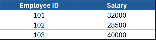
You want to combine the Salary column from Table 2 into Table 1, so each employee’s record includes their pay.

‍

Step 2: Writing a Basic VLOOKUP Formula

In Table 1, next to the “Department” column, create a new column called Salary. Then enter the following formula in the first row (e.g., cell D2):

=VLOOKUP(A2, $G$2:$H$4, 2, FALSE)


Here’s what’s happening:

• A2 – the Employee ID you want to look up.
• $G$2:$H$4 – the range containing the data from Table 2 (the lookup table).
• 2 – the column number in that range that contains the salary.
• FALSE – tells Excel to find an exact match.

When you press Enter, Excel finds the Employee ID in Table 2 and returns the matching salary.

Copy the formula down the column, and your list is complete.

‍

Step 3: Understanding Absolute References

Notice the dollar signs ($) in $G$2:$H$4. These make the cell references absolute, meaning they don’t change when you copy the formula down.

If you forget to use $, Excel might look in the wrong rows as you copy the formula, causing incorrect results.

You can quickly toggle between reference types by selecting the range in your formula and pressing F4.

‍

Step 4: Using VLOOKUP Across Worksheets

VLOOKUP doesn’t have to stay on the same sheet. You can easily pull data from another worksheet.

Example:

=VLOOKUP(A2, 'Salary Data'!$A$2:$B$100, 2, FALSE)


The 'Salary Data'! part tells Excel to look on a sheet named “Salary Data.”

‍

Step 5: Using VLOOKUP Across Workbooks

You can even reference another workbook:

=VLOOKUP(A2, '[CompanyData.xlsx]Sheet1'!$A$2:$B$100, 2, FALSE)


When you do this, Excel creates a link between the files. If you move or rename the source file, the formula may break — so keep linked workbooks organised in one folder if possible.

‍

Step 6: Handling Missing Data

Sometimes, a lookup value isn’t found in the table. In that case, VLOOKUP returns #N/A.

To make your sheet more readable, you can wrap the formula in an IFERROR function:

=IFERROR(VLOOKUP(A2, $G$2:$H$4, 2, FALSE), "Not Found")


Now, if the value doesn’t exist, Excel will display “Not Found” instead of an error message.

‍

Step 7: Using Approximate Matches

Although exact matches are most common, VLOOKUP can also find approximate matches (useful for things like grading or pricing tiers).

Set the fourth argument to TRUE or leave it blank:

=VLOOKUP(B2, $A$2:$B$10, 2, TRUE)


Important: For approximate matches to work correctly, the first column of your lookup table must be sorted in ascending order.

Example:

VLOOKUP will find the largest value less than or equal to the lookup value — ideal for assigning grades.

‍

Step 8: Combining Data from Multiple Columns

You can also combine data before using VLOOKUP by creating a helper column.

Example: Suppose you need to match on both First Name and Last Name.

1. In the source table, insert a new column.
2. In that column, use:

=A2 & " " & B2


This joins the two names with a space in between.
3. Use the same formula in the other table to create matching keys.
4. Use VLOOKUP on the helper column.

‍

Step 9: Replacing VLOOKUP with XLOOKUP (Optional)

If you’re using Microsoft 365 or Excel 2021, there’s a new function called XLOOKUP. It’s more flexible than VLOOKUP and doesn’t require your lookup column to be first.

Example:

=XLOOKUP(A2, $G$2:$G$4, $H$2:$H$4, "Not Found")


‍

XLOOKUP is faster and easier to maintain, but VLOOKUP is still widely used and supported in older versions of Excel.

‍

Step 10: Common Errors and Fixes

‍

Step 11: VLOOKUP Best Practices

• Always use absolute references for table ranges.
• Avoid inserting new columns in the middle of lookup tables (it can break formulas).
• Use named ranges (e.g., EmployeeList) instead of cell references for clarity.
• Combine VLOOKUP with IFERROR for cleaner reports.
• Test with a small sample before applying to large datasets.

‍

Step 12: Real-World Scenarios

1. Merging Client Lists – Combine customer data from two systems using a common Customer ID.
2. Tracking Inventory – Match stock numbers to product descriptions.
3. HR Reporting – Add employee names or departments to payroll exports.
4. Sales Analysis – Bring product categories into a sales report for deeper insights.

‍

Step 13: When VLOOKUP Isn’t Enough

For complex models or large data sets, consider alternatives:

• INDEX-MATCH – More flexible and reliable for large tables.
• XLOOKUP – The modern replacement for VLOOKUP.
• Power Query – Ideal for merging multiple data sources without formulas.

‍

Conclusion

VLOOKUP is one of Excel’s most valuable functions for anyone who works with multiple data sets. It saves time, reduces manual matching, and helps you build clear, professional reports.

In this article, we covered:

• The syntax and structure of VLOOKUP
• Exact and approximate matches
• Handling errors with IFERROR
• Using helper columns and combining data
• Best practices and common pitfalls

Once you’ve mastered VLOOKUP, you’ll be ready to tackle even more advanced lookup functions like INDEX-MATCH, XLOOKUP, and Power Query joins.

If you’d like to build these skills with expert guidance, ExperTrain offers hands-on Excel courses for every level:

• Excel Introduction – Learn the fundamentals of Excel and basic formulas.
• Excel Intermediate – Master VLOOKUP, logical functions, and essential data tools.
• Excel Advanced – Learn advanced lookup formulas, data analysis, and automation.
• Excel Power User – Explore data modelling, advanced functions, and Power Query integration.

With the right training, you can take your Excel skills from basic lookups to complete data management mastery.

‍