How to Use INDEX and MATCH in Excel

Introduction

If you’ve used VLOOKUP and hit problems (like not being able to look left or your columns breaking when you insert a new one), it’s time to learn INDEX + MATCH. This pair of functions is more flexible, more reliable, and works with both vertical and horizontal lookups. With a few simple examples, you’ll be able to fetch the exact value you need from any table without rearranging your data.

In this guide you’ll learn:

• What INDEX and MATCH do, and why they work so well together
• How to build vertical, horizontal, and two-way lookups
• How to do left lookups (which VLOOKUP can’t do)
• How to match exact, approximate, wildcard, and multiple criteria
• How to add error handling and data validation for clean results
• Power tips: structured references, dynamic ranges, duplicate handling, and performance

We’ll use plain language and step-by-step examples so you can follow along in any modern version of Excel (Microsoft 365 or standalone).

What INDEX and MATCH do (in one minute)

• INDEX(array, row_num, [column_num]) returns the value at a specific row and column inside a range.
  Think of INDEX as “give me the value at coordinates (row, column).”
• MATCH(lookup_value, lookup_array, [match_type]) returns the position of a value within a range.
  Think of MATCH as “tell me the row (or column) number where this thing is.”

Together:

1. Use MATCH to find which row/column contains your key.
2. Feed that position into INDEX to return the value from the table.

Quick example: a vertical lookup with INDEX + MATCH

Imagine a simple price list:

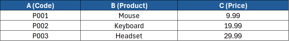
You want the Price for product code in F2.

Formula (in G2):

=INDEX(C:C, MATCH(F2, A:A, 0))


• MATCH(F2, A:A, 0) finds the row of the code in column A (0 = exact match).
• INDEX(C:C, …) returns the value from column C at that row.

This is the classic “look left” win: your lookup column (A) is left of the return column (C). VLOOKUP struggles here; INDEX + MATCH handles it easily.

Syntax notes you’ll use often

• MATCH(..., 0) = exact match (most common for IDs/text).
• MATCH(..., 1) = approximate (lookup array must be sorted ascending).
• MATCH(..., -1) = approximate descending (array sorted descending).
• INDEX(range, row, column) – if you give INDEX a single column, you only need the row. If you give a whole table, you can supply both row and column.

Two-way lookup (row by one field, column by another)

Say you have a small sales table:

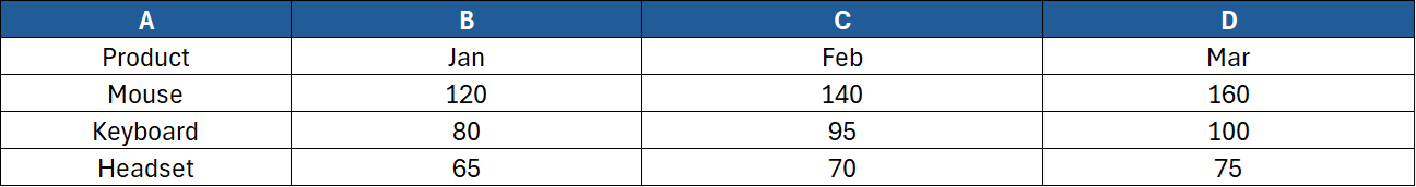
• Product name in G2 (e.g., “Keyboard”)
• Month in H2 (e.g., “Feb”)

Formula (in I2):

=INDEX(B2:D4, MATCH(G2, A2:A4, 0), MATCH(H2, B1:D1, 0))


• The first MATCH finds the row for the product.
• The second MATCH finds the column for the month.
• INDEX returns the cell at that row and column.

Horizontal lookup (MATCH across columns)

If your headers run across the top and you want a figure from a single row, switch the roles:

=INDEX(2:2, MATCH("Mar", 1:1, 0))


• Finds the column of “Mar” in row 1, then returns the corresponding value from row 2.

Handle missing values nicely with IFERROR

If the lookup value doesn’t exist, MATCH returns #N/A. Wrap your formula with IFERROR for user-friendly messages:

=IFERROR(INDEX(C:C, MATCH(F2, A:A, 0)), "Not found")


For dashboards, you might return a blank:

=IFERROR(INDEX(C:C, MATCH(F2, A:A, 0)), "")


Wildcard lookups (contains / starts with)

You can search partial text with * (any characters) and ? (single character).
Example: find product containing the word in F2:

=INDEX(C:C, MATCH("*" & F2 & "*", B:B, 0))


• If F2 = "board", MATCH finds “Keyboard” in column B.

Tip: If your lookup value might contain ? or * literally, escape them: replace ~? or ~*.

Multiple-criteria lookup (no helper column)

Suppose you need the Price for Product + Region. You can build a boolean array and use MATCH with it.

Columns:

• A: Product
• B: Region
• C: Price
  Inputs:
• F2: Product (e.g., “Keyboard”)
• G2: Region (e.g., “EMEA”)

Formula (dynamic array Excel):

=INDEX(C:C, MATCH(1, (A:A=F2)*(B:B=G2), 0))


• (A:A=F2) returns a TRUE/FALSE array.
• (B:B=G2) returns a TRUE/FALSE array.
• Multiplying them gives 1 only where both are TRUE.
• MATCH finds the position of that 1.

In older Excel, confirm array formulas with Ctrl+Shift+Enter. In Microsoft 365, just press Enter.

First match vs last match (duplicate keys)

First match is what MATCH returns by default.
To find the last match in a column (e.g., the latest transaction for an ID), you can flip the search direction:

Option A (LOOKUP trick):

=LOOKUP(2, 1/(A:A=F2), C:C)


• 1/(A:A=F2) creates an array of 1s (match) and #DIV/0! (no match).
• LOOKUP(2, …) walks to the last numeric 1 and returns the aligned value from C:C.

Option B (XMATCH if available):

=INDEX(C:C, XMATCH(F2, A:A, 0, -1))


• The 4th argument -1 searches last-to-first. (XMATCH is in newer Excel.)

Approximate lookups (bands and grades)

To return a result by band (e.g., commission rate by threshold), sort the lookup column ascending and use MATCH(…,1):

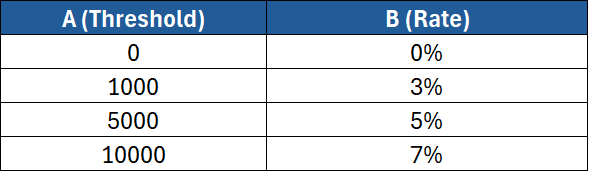
Sales value in F2 → Rate:

=INDEX(B:B, MATCH(F2, A:A, 1))


If F2 is 7,200, MATCH returns the position of 5,000 (the largest value ≤ sales), and INDEX returns 5%.

For descending bands, sort descending and use MATCH(…, -1).

Case-sensitive lookups (advanced)

MATCH ignores case. To make it case-sensitive, use EXACT inside an array:

=INDEX(C:C, MATCH(TRUE, EXACT(A:A, F2), 0))


• Confirm with Ctrl+Shift+Enter in older Excel.
• In Microsoft 365, Enter is enough.

Use named ranges and Excel Tables for safer formulas

Hard-coding whole columns works, but named ranges or Tables make formulas more robust and faster.

Named range example

Select A2:A100 (codes) → Formulas > Define Name → Codes.
Select C2:C100 (prices) → name Prices. Then:

=INDEX(Prices, MATCH(F2, Codes, 0))


Excel Table example

• Select your data → Insert > Table (tick “My table has headers”).
• Rename the table to tblProducts.
• Structured references:

=INDEX(tblProducts[Price], MATCH([@Code], tblProducts[Code], 0))


Tables auto-expand as you add rows, so your lookup keeps working.

Dynamic ranges with INDEX (no volatile OFFSET)

To define a range that grows, you can use INDEX to reference the last used row:

=Sheet1!$A$2:INDEX(Sheet1!$A:$A, COUNTA(Sheet1!$A:$A))


• This returns A2: A{last non-blank}.
• Use in Name Manager, then refer to the name in your formulas.

INDEX-based ranges are non-volatile (usually faster than OFFSET).

Debug faster with F9 and Evaluate Formula

• Highlight part of a formula (e.g., just the MATCH) and press F9 to see what it returns. Press Esc to cancel.
• Use Formulas > Evaluate Formula to step through a complex expression.

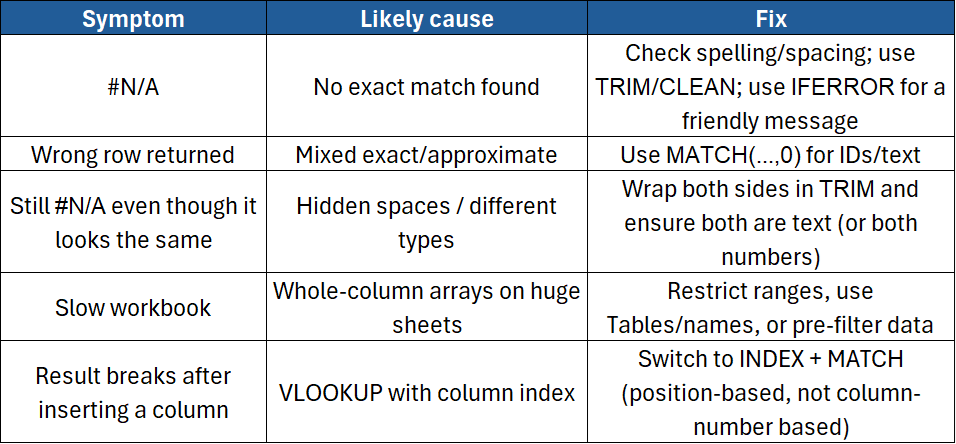
Common mistakes and how to fix them

INDEX + MATCH vs XLOOKUP (which should I use?)

If you have XLOOKUP, it combines the two functions and is simpler to read:

=XLOOKUP(F2, A:A, C:C, "Not found")


However, INDEX + MATCH is still worth learning because:

• It works on older Excel versions
• It’s very flexible for two-way and multi-criteria lookups
• It helps you understand positions vs values, which is useful in many formulas

Worked example: multi-criteria two-way lookup

Goal: Return Unit Price by Product and Region from a table.

Headers (row 1): Product | Region | Unit Price | Discount
Inputs: H2 = Product, H3 = Region

Formula (Unit Price):

=INDEX(C2:C100, MATCH(1, (A2:A100=H2)*(B2:B100=H3), 0))


Add IFERROR for user-friendly output:

=IFERROR(INDEX(C2:C100, MATCH(1, (A2:A100=H2)*(B2:B100=H3), 0)), "No match")


To turn this into a two-way lookup (e.g., choose between returning “Unit Price” or “Discount” based on a header in H4):

=INDEX(C2:D100, MATCH(1, (A2:A100=H2)*(B2:B100=H3), 0), MATCH(H4, C1:D1, 0))


Now H4 can be “Unit Price” or “Discount”, and the formula returns the correct column.

Data validation to reduce errors

Help users enter valid keys:

• Data > Data Validation
• Allow: List (point to the list of products or codes)
• Or Custom rules for patterns (e.g., codes starting with “P”)

Cleaner inputs = fewer #N/A lookups.

Performance tips

• Use Tables or limit ranges (e.g., A2:A5000 instead of A:A) on very large sheets.
• Avoid stacking volatile functions (e.g., INDIRECT/OFFSET) in large arrays.
• Pre-compute helper columns if a single giant formula is slow.
• Consider dynamic arrays (FILTER, UNIQUE) to pre-filter data before lookup where appropriate.

Security and sharing tips

• If lookups reference a protected sheet or external workbook, ensure recipients have permissions.
• For external links, use File > Info > Edit Links (or Data > Queries & Connections) to review connections before sharing.

Conclusion

INDEX + MATCH gives you flexible, reliable lookups that don’t break when your data changes. You can match on exact values, partial text, multiple criteria, or even the last occurrence—then return a value from any column or row. With error handling and structured references, your spreadsheets will be cleaner, faster, and easier to maintain.

If you’d like hands-on practice with live examples and expert feedback, check out our Excel courses:

• Excel Introduction – Core functions and clean formulas.
• Excel Intermediate – Lookups (INDEX/MATCH), structured references, and tables.
• Excel Advanced – Array formulas, dynamic arrays, advanced error handling.
• Excel Power User: Mastering Complex Functions and Data Models – Multi-criteria logic, performance tuning, and real-world modelling.

‍