How to Clean Data Using Power Query in Excel

Introduction

Messy data wastes time. Extra spaces, wrong cases, mixed date formats, columns that should be rows, rows that should be columns, and files that arrive slightly different every week. Power Query in Excel fixes this. You point Power Query at your data, click through the steps you need, and Excel remembers those steps. Next time the data changes, you just click Refresh.

In this guide you will learn how to:

• Import data from common sources
• Understand the Power Query Editor and the Applied Steps list
• Fix types, headers, blanks, and errors
• Trim, split, merge, and standardise text
• Remove duplicates and keep the rows you need
• Unpivot and pivot to reshape tables
• Group and summarise
• Merge and append multiple tables
• Combine a folder of files
• Build parameters and tidy query structure
• Refresh safely and avoid common problems

Everything here uses modern Excel with Power Query built in.

What is Power Query

Power Query is a tool in Excel that helps you get data, clean it, and shape it without writing formulas in the worksheet. You use a friendly editor. Each change you make becomes a step. Excel stores those steps in a small script behind the scenes. You can reuse the same steps every time the raw data updates.

Where to find it

• Data tab in Excel
• Buttons: Get Data, From Table/Range, From Text/CSV, From Folder, From Web, From Database

When you load data into Power Query, the Power Query Editor opens in a separate window.

The Power Query Editor at a glance

• Queries pane (left): list of all queries in the file
• Data preview (centre): a sample of your table
• Ribbon (top): Home, Transform, Add Column, View
• Applied Steps (right): every change you make, in order

You can click a step to go back in time, rename a step, reorder steps with care, or delete a step if needed.

Golden rules before you start

1. Start with a table or a clear range when pulling from the sheet. Use Format as Table if possible.
2. Use correct types early. If a column is a date, set it as Date.
3. Rename columns to friendly names. It helps later steps.
4. Keep steps small. One action per step makes it easier to debug.
5. Avoid changing column order unless you must. Match on names instead of positions where possible.

Import data the easy way

From a table or range

Select a cell in your data on the worksheet and choose Data > From Table/Range. Tick My table has headers if true.

From a CSV

Use Data > Get Data > From File > From Text/CSV. Power Query detects the delimiter. Click Transform Data to open the editor.

From a folder of files

Use Data > Get Data > From File > From Folder to combine many files that share the same layout. This is perfect for monthly drops.

First clean-up pass: types, headers, blanks

1. Promote headers
   If the first row contains headers, choose Home > Use First Row as Headers.
2. Set data types
   Select each column and choose a type from the icon in the header: Whole Number, Decimal Number, Date, Text, True/False.
   Getting types right early avoids later errors.
3. Remove top or bottom rows
   Home > Remove Rows > Remove Top Rows or Remove Bottom Rows for banner lines or footers.
4. Remove blanks
   Filter the column to remove nulls or use Home > Remove Rows > Remove Blank Rows where suitable.
5. Replace error values
   Use Home > Replace Errors or filter Error from the column drop-down and decide how to handle them.

Text clean-up: trim, clean, case, split, merge

Trim and clean

• Transform > Format > Trim removes space at the start and end.
• Transform > Format > Clean removes non-printing characters.

Fix capitalisation

• Transform > Format > Capitalize Each Word
• Lowercase or Uppercase if that suits your data.

Replace values

• Transform > Replace Values to swap quick strings like “N/A” to null.

Split columns

• Transform > Split Column > By Delimiter (comma, space, dash).
• Split By Number of Characters for fixed width feeds.
• Choose At the left-most delimiter, Each occurrence, or At the right-most delimiter.

Merge columns

• Transform > Merge Columns, pick a separator like space or dash. Good for building a full name from first and last.

Tip: If you use split then merge often, consider building a Custom Column instead to keep control.

Numbers and dates: standardise and fix

• Change type to Decimal or Whole as needed.
• Transform > Standard > Multiply/Divide to fix scale (for example if cents arrive as whole units).
• Transform > Date to extract Year, Month, Quarter, Start of Month, End of Month.
• Transform > Using Locale to convert a text date where the incoming format uses a different region.

Keep the rows you want

• Filter from the column drop-down.
• Text Filters like Contains, Begins With.
• Number Filters like Greater Than.
• Date Filters like In This Month.
• Home > Remove Rows > Remove Duplicates on one or more columns to keep the first occurrence.
• Keep Rows options are useful too. You can Keep Top Rows for samples or Keep Range of Rows.

Unpivot and pivot: reshape for analysis

Power Query makes it easy to tidy cross-tab data into tidy columns.

Unpivot (make columns into rows)

Use when you have one column per month or per category and you want a single Attribute column and a single Value column.

1. Select the identifier columns you want to keep, like Customer and Product.
2. Transform > Unpivot Columns > Unpivot Other Columns.
3. Rename Attribute to Month, Value to a meaningful measure name.

Pivot (make rows into columns)

Use when you need one column per category.

1. Select the column that holds the future headers, then Transform > Pivot Column.
2. Choose the Values Column and an Aggregate such as Sum or Count.

Group and summarise

Home > Group By lets you sum, count, average, and more by one or more keys.
For example, group by Customer and Month and sum Sales.
You can add multiple aggregations in one step.

Merge and append: join many tables together

Append (stack tables)

Use when two or more tables have the same columns and you want one long table.

• Home > Append Queries
• Choose Two tables or Three or more tables

Merge (join tables by key)

Use when you want to bring lookup columns across, similar to VLOOKUP but more flexible.

1. Home > Merge Queries
2. Pick the two tables and choose the matching key columns
3. Choose the Join kind:
   • Left Outer keeps all rows from the first table
   • Inner keeps matches only
   • Right Outer, Full Outer, Left Anti (only non-matches), Right Anti
4. Expand the new column to pick the fields you want to bring in

Tip: Always check the join matches by looking at the row counts before and after.

Combine a folder of monthly files

This saves loads of time when you receive one file per period with the same layout.

1. Get Data > From Folder
2. Choose the folder path that holds all the files
3. Click Combine. Power Query will show a preview using a sample file
4. If the data starts on row 7 or has a header line to skip, fix it in the Transform Sample File query. This change will apply to all files
5. The output is one combined table
6. Keep the folder clean. New files dropped into the folder appear after Refresh

Conditional columns and custom logic

Conditional Column

Add Column > Conditional Column lets you build simple IF rules:

• If Status equals “Closed” then 0 else Amount
• If Score is ≥ 90 then “A”, else if ≥ 80 then “B”, else “C”

Custom Column

For more control you can write a short M expression. Here are a few handy patterns:

Proper case a name with extra trimming:

= Text.Proper(Text.Trim([Name]))


Extract a 3-letter month from a Date column:

= Date.ToText([OrderDate], "MMM")


Safe divide that avoids errors when the denominator is zero:

= try [Sales] / [Units] otherwise null


Turn blanks to nulls in a text column:

= if [Code] = "" then null else [Code]


Error handling that keeps refreshes calm

Errors can appear when types change or data is missing. You have options:

• Transform > Replace Errors to set a default value
• Add Column > Invoke Custom Function combined with try ... otherwise in M to handle risky steps
• Filter out Error rows if you do not need them, or send them to a separate query for review

Step order and performance tips

• Remove columns you do not need early. Less data means faster steps later.
• Change types near the top. Many transforms rely on correct types.
• Group and summarise before merging when possible. Joining smaller tables is faster.
• Avoid repeated sorts. Sort once if you must.
• Prefer built-in transformations over complex custom code when performance matters.
• Turn off column profiling on very large tables if the editor feels slow: View > Column quality toggles.

Parameters for paths, dates, and switches

Parameters make queries reusable.

• Manage Parameters > New Parameter
• Store things like a folder path, a start date, or a feature toggle
• Use the parameter inside steps such as Source or inside filters
• Change the parameter value without editing the M code

Name queries and keep structure tidy

Use short, clear names:

• stg_SalesCSV for a staging query that holds raw import
• dim_Customer for a cleaned lookup
• fact_Sales for the final sales table
• fx_CleanText for a reusable custom function

Keep staging queries as Connection only if you do not need them on the sheet.

Load options: Table or Data Model

When you click Close & Load, Excel creates a table on a new sheet.
If you plan to build a PivotTable or connect to Power Pivot, choose Close & Load To… then pick Only Create Connection and Add this data to the Data Model. This avoids heavy sheet tables and keeps files smaller.

Refresh and privacy settings

• Data > Refresh All reloads everything
• Right-click a query in the Queries pane to refresh a single table
• On the Query Properties, you can set Refresh every X minutes or Refresh data when opening the file
• Privacy levels protect you from mixing data across sources in ways that might leak information. If your sources are trusted and you see a privacy warning, set appropriate levels under Data > Get Data > Query Options > Privacy or talk to IT

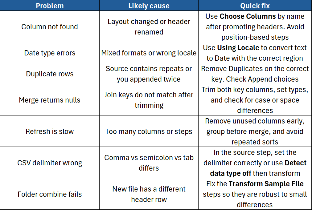
Troubleshooting guide

Example cleaning flow you can copy

Goal: Clean a monthly CSV of sales and load a tidy table.

1. Get Data > From Text/CSV and click Transform Data
2. Use First Row as Headers
3. Remove Top Rows = 1 if there is a banner line
4. Choose Columns to keep only: Date, Product, Customer, Units, Amount
5. Set types: Date, Text, Text, Whole Number, Decimal Number
6. Trim and Clean on Product and Customer
7. Add a Conditional Column for Band: Units ≥ 100 is “Large”, else “Standard”
8. Remove Duplicates on Date, Product, Customer if needed
9. Close & Load To… create a Table on a sheet called Sales_Clean
10. Next month, drop the new CSV in the same place and click Refresh

Best practice checklist

• Use Format as Table or a clean CSV as your source
• Promote headers and set types early
• Trim, clean, and standardise text
• Remove extra columns and duplicates
• Use Unpivot for month columns and other cross-tabs
• Group before merge where it makes sense
• Build Parameters for paths and filters
• Keep queries and steps well named
• Load to the Data Model when you plan to analyse with PivotTables
• Refresh and test after each big change

Conclusion

Power Query turns messy data into tidy tables you can trust. You record your cleaning steps once, then refresh as often as you like. It is faster than manual fixes and more reliable than one-off formulas. With a few clicks you can trim, split, unpivot, merge, and combine files. Follow the steps in this guide to build a repeatable data pipeline in Excel.

‍